2. Dictionary Inputs#
In the previous example, the model parameters were built from a ‘.yaml’ file. In some cases, the functional parameters are relatively complex and can be challenging to specify in the ‘.yaml’ format. Therefore, the model can also be constructed using a dictionary, as demonstrated below.
2.1. Import Modules#
1import thevenin
2import numpy as np
2.2. Define the Parameters#
In addition to the open circuit voltage (ocv), all circuit elements (i.e., R0, R1, C1, etc.) must be specified as functions. While OCV is only a function of the state of charge (soc, -), the circuit elements are function of both soc and temperature (T_cell, K). It is important that these are the only inputs to the functions and that the inputs are given in the correct order.
The functions below come from fitting the equivalent circuit model to a 75 Ah graphite-NMC battery made by Kokam. Fits were performed using charge and discharge pulses from HPPC tests done at multiple temperatures. The soc was assumed constant during a single pulse and each resistor and capacitor element was fit as a constant for a given soc/temperature condition. Expressions below come from AI-Batt, which is an open-source software capable of semi-autonomously identifying algebraic expressions that map inputs (soc and T_cell) to outputs (R0, R1, C1).
 1stressors = {'q_dis': 1.}
 2
 3
 4def calc_xa(soc: float) -> float:
 5    return 8.5e-3 + soc*(7.8e-1 - 8.5e-3)
 6
 7
 8def calc_Ua(soc: float) -> float:
 9    xa = calc_xa(soc)
10    Ua = 0.6379 + 0.5416*np.exp(-305.5309*xa) \
11                + 0.0440*np.tanh(-1.*(xa-0.1958) / 0.1088) \
12                - 0.1978*np.tanh((xa-1.0571) / 0.0854) \
13                - 0.6875*np.tanh((xa+0.0117) / 0.0529) \
14                - 0.0175*np.tanh((xa-0.5692) / 0.0875)
15
16    return Ua
17
18
19def normalize_inputs(soc: float, T_cell: float) -> dict:
20    inputs = {
21        'T_norm': T_cell / (273.15 + 35.),
22        'Ua_norm': calc_Ua(soc) / 0.123,
23    }
24    return inputs
25
26
27def ocv_func(soc: float) -> float:
28    coeffs = np.array([
29        1846.82880284425, -9142.89133579961, 19274.3547435787, -22550.631463739,
30        15988.8818738468, -7038.74760241881, 1895.2432152617, -296.104300038221,
31        24.6343726509044, 2.63809042502323,
32    ])
33    return np.polyval(coeffs, soc)
34
35
36def R0_func(soc: float, T_cell: float) -> float:
37    inputs = normalize_inputs(soc, T_cell)
38    T_norm = inputs['T_norm']
39    Ua_norm = inputs['Ua_norm']
40
41    b = np.array([4.07e12, 23.2, -16., -47.5, 2.62])
42
43    R0 = b[0] * np.exp( b[1] / T_norm**4 * Ua_norm**(1/4) ) \
44              * np.exp( b[2] / T_norm**4 * Ua_norm**(1/3) ) \
45              * np.exp( b[3] / T_norm**0.5 ) \
46              * np.exp( b[4] / stressors['q_dis'] )
47
48    return R0
49
50
51def R1_func(soc: float, T_cell: float) -> float:
52    inputs = normalize_inputs(soc, T_cell)
53    T_norm = inputs['T_norm']
54    Ua_norm = inputs['Ua_norm']
55
56    b = np.array([2.84e-5, -12.5, 11.6, 1.96, -1.67])
57
58    R1 = b[0] * np.exp( b[1] / T_norm**3 * Ua_norm**(1/4) ) \
59              * np.exp( b[2] / T_norm**4 * Ua_norm**(1/4) ) \
60              * np.exp( b[3] / stressors['q_dis'] ) \
61              * np.exp( b[4] * soc**4 )
62
63    return R1
64
65
66def C1_func(soc: float, T_cell: float) -> float:
67    inputs = normalize_inputs(soc, T_cell)
68    T_norm = inputs['T_norm']
69    Ua_norm = inputs['Ua_norm']
70
71    b = np.array([19., -3.11, -27., 36.2, -0.256])
72
73    C1 = b[0] * np.exp( b[1] * soc**4 ) \
74              * np.exp( b[2] / T_norm**4 * Ua_norm**(1/2) ) \
75              * np.exp( b[3] / T_norm**3 * Ua_norm**(1/3) ) \
76              * np.exp( b[4] / stressors['q_dis']**3 )
77
78    return C1
2.3. Construct a Model#
The model is constructed below using all necessary keyword arguments. You can see a list of these parameters using help(thevenin.Model).
 1params = {
 2    'num_RC_pairs': 1,
 3    'soc0': 1.,
 4    'capacity': 75.,
 5    'mass': 1.9,
 6    'isothermal': False,
 7    'Cp': 745.,
 8    'T_inf': 300.,
 9    'h_therm': 12.,
10    'A_therm': 1.,
11    'ocv': ocv_func,
12    'R0': R0_func,
13    'R1': R1_func,
14    'C1': C1_func,
15}
16
17model = thevenin.Model(params)
2.4. Build an Experiment#
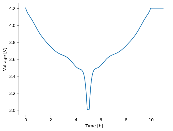
Experiments are built using the Experiment class. An experiment starts out empty and is then constructed by adding a series of current-, voltage-, or power-controlled steps. Each step requires knowing the control mode/units, the control value, a relative time span, and limiting criteria (optional). Control values can be specified as either constants or dynamic profiles with sinatures like f(t: float) -> float where t is the relative time of the new step, in seconds. The experiment below discharges at a nominal C/5 rate for up to 5 hours. A limit is set such that if the voltage hits 3 V then the next step is triggered early. Afterward, the battery rests for 10 min before charging at C/5 for 5 hours or until 4.2 V is reached. The final step is a 1 hour voltage hold at 4.2 V.
Note that the time span for each step is constructed as (t_max: float, dt: float) which is used to determine the time array as tspan = np.arange(0., t_max + dt, dt). You can also construct a time array given (t_max: float, Nt: int) by using an integer instead of a float in the second position. In this case, tspan = np.linspace(0., t_max, Nt). To learn more about building an experiment, including which limits are allowed and/or how to adjust solver settings on a per-step basis, see the documentation help(thevenin.Experiment).
1expr = thevenin.Experiment()
2expr.add_step('current_A', 15., (5.*3600., 60.), limits=('voltage_V', 3.))
3expr.add_step('current_A', 0., (600., 5.))
4expr.add_step('current_A', -15., (5.*3600., 60.), limits=('voltage_V', 4.2))
5expr.add_step('voltage_V', 4.2, (3600., 60.))
2.5. Run the Experiment#
Experiments are run using either the run method, as shown below, or the run_step method. The difference between the two is that the run method will run all experiment steps with one call. If you would prefer to run the discharge first, perform an analysis, and then run the rest, etc. then you will want to use the run_step method. In this case, you should always start with step 0 and then run the following steps in order. When you use run_step the models internal state is saved at the end of each step. Therefore, after all steps have been run, you should run the pre method to pre-process the model back to its original initial state. All of this is handled automatically in the run method.
Regardless of how you run your experiment, the return value will be a solution instance. Solution instances each contain a vars attribute which contains a dictionary of the output variables. Keys are generally self descriptive and include units where applicable. To quickly plot any two variables against one another, use the plot method with the two keys of interest specified for the x and y variables of the figure. Below, time (in hours) is plotted against voltage.
1soln = model.run(expr)
2soln.plot('time_h', 'voltage_V')