Tuning ECM Models with Online Estimation

This tutorial describes how to monitor battery health with online estimation if you already know an Equivalent Circuit Model (ECM) for its behavior.

Load Example Data

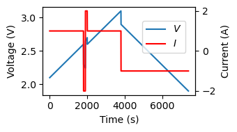
We’ll use the data from a simple battery model as a demonstration

from pathlib import Path
from shutil import copyfileobj
import requests

data_url = 'https://github.com/ROVI-org/battery-data-toolkit/raw/refs/heads/main/tests/files/example-data/single-resistor-complex-charge_from-discharged.hdf'
data_path = Path('files') / 'complex-cycle-data.hdf'

if not data_path.is_file():
    data_path.parent.mkdir(exist_ok=True)
    data_path.write_bytes(requests.get(data_url).content)

Load it as a battery-data-toolkit dataset object

from battdat.data import CellDataset
data = CellDataset.from_hdf(data_path)

/home/lward/miniconda3/envs/moirae/lib/python3.10/site-packages/battdat/data.py:57: UserWarning: Metadata was created in a different version of battdat. supplied=0.4.0, current=0.4.1.
  warnings.warn(f'Metadata was created in a different version of battdat. supplied={supplied_version}, current={__version__}.')

%matplotlib inline
from matplotlib import pyplot as plt
fig, ax = plt.subplots(figsize=(3.5, 2.))

raw_data = data.raw_data
ax.plot(raw_data['test_time'], raw_data['voltage'], label='$V$')
ax.set_xlabel('Time (s)')
ax.set_ylabel('Voltage (V)')

ax2 = ax.twinx()
ax2.plot(raw_data['test_time'], raw_data['current'], color='red', label='$I$')
ax2.set_ylabel('Current (A)')

fig.legend(loc=(0.6, 0.6))
fig.tight_layout()

Recreate the ECM Parameters with Moirae

Moirae includes a Python implementation of a Thevenin ECM.

Define the parameters for the ECM model as Moirae-compatible Health parameter objects

All components of the model will eventually be combined to form a ECMASOH object, and we’ll only show the basic ones here (OCV, capacity, serial resistance)

Here, we assume that good guesses for parameters are already known. Use extractors to make guesses otherwise.

from moirae.models.ecm import ECMASOH
for name, field in ECMASOH.model_fields.items():
    if name != "updatable":
        print(name, field.description)

q_t Maximum theoretical discharge capacity (Qt).
ce Coulombic efficiency (CE)
ocv Open Circuit Voltage (OCV)
r0 Series Resistance (R0)
c0 Series Capacitance (C0)
rc_elements Tuple of RC components
h0 Hysteresis component

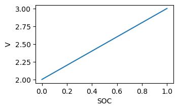
The OCV is described using SOC-dependent variable defined using interpolation points. Interpolation points are assumed to be evenly-spaced across [0, 1] and the values at each point are defined as “base values”

from moirae.models.ecm.components import OpenCircuitVoltage, SOCInterpolatedHealth
ocv = OpenCircuitVoltage(
    ocv_ref=SOCInterpolatedHealth(base_values=[2, 3.])
)

import numpy as np
fig, ax = plt.subplots(figsize=(3.5, 2.))

soc = np.linspace(0., 1, 32)[None, :]
v = ocv(soc)
ax.plot(soc.flatten(), v.flatten())

ax.set_xlabel('SOC')
ax.set_ylabel('V')

Text(0, 0.5, 'V')

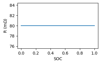
The resistance can be dependent on both SOC and temperature, but we’ll choose to make it insensitive to both by defining only a single interpolation point.

from moirae.models.ecm.components import Resistance
r0 = Resistance(base_values=[0.080])

import numpy as np
fig, ax = plt.subplots(figsize=(3.5, 2.))

soc = np.linspace(0., 1, 32)[None, :]
r = r0.get_value(soc)
ax.plot(soc.flatten(), r.flatten() * 1000)

ax.set_xlabel('SOC')
ax.set_ylabel('R (m$\\Omega$)')

Text(0, 0.5, 'R (m$\\Omega$)')

Capacity is defined as a “max theoretical capacity,” which allows for capacity to change with parameters such as temperature

from moirae.models.ecm.components import MaxTheoreticalCapacity
q_t = MaxTheoreticalCapacity(base_values=1.)

Finally, combine them together

asoh = ECMASOH(
    q_t=q_t,
    ocv=ocv,
    r0=r0,
)

We’re now ready to fit the parameters

Run the model

Let’s start by running the model using the same input currents as provided in the data. Moirae provides a simple interface to running a model given input data from a battery-data-toolkit BatteryDataset.

The first step is to make an interface to running the ECM.

from moirae.models.ecm import EquivalentCircuitModel
model = EquivalentCircuitModel()

We then create a “transient state” which defines the initial state of charge of the system.

from moirae.models.ecm.transient import ECMTransientVector
state = ECMTransientVector.from_asoh(asoh)
state

ECMTransientVector(soc=array([[0.]]), q0=None, i_rc=array([], shape=(1, 0), dtype=float64), hyst=array([[0.]]))

Then run it

from moirae.interface import run_model
output = run_model(
    model=model,
    dataset=data,
    asoh=asoh,
    state_0=state
)

%matplotlib inline
fig, ax = plt.subplots(figsize=(3.5, 2.))

ax.plot(raw_data['test_time'], raw_data['voltage'], 'k--', label='Actual')
ax.plot(raw_data['test_time'], output['terminal_voltage'], color='r', label='Model')
ax.set_xlabel('Time (s)')
ax.set_ylabel('Voltage (V)')

fig.legend()
fig.tight_layout()

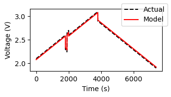
The result is close, but not quite the on point. We might have an issue with the resistance.

Fitting ASOH with Online State Estimation

Online state estimation works by adjusting the estimates for the state of a dynamic system based on discrepancies between values predicted by a model for that system and what is actually measured. The “online” portion in the algorithm refers to it why it works: gradually adjusting with every new measurement.

The ‘online estimator’ classes in Moirae define online estimation algorithms. For simplicity, we’ll make one which estimates the resistance value and the SOC.

Start by marking the interpolation point for serial resitance (“r0.base_values”) as updatable.

asoh.mark_updatable('r0.base_values')
asoh.updatable_names

('r0.base_values',)

Then define uncertainties in the transient state (SOC and hysteresis values) and the resistance. Each are expressed using covariance matrices.

asoh_covar = np.array([[0.001]])
tran_covar = np.diag([0.0001, 1e-7])

The state estimator requires estimates for the noise in the model and measurement. We’ll make them all rather small

voltage_err = 1.0e-03  # mV voltage error
noise_sensor = ((voltage_err / 2) ** 2) * np.eye(1)
noise_asoh = 1.0e-10 * np.eye(asoh_covar.shape[0])
noise_tran = 1.0e-08 * np.eye(2)

from moirae.estimators.online.joint import JointEstimator
from moirae.models.ecm.ins_outs import ECMInput
estimator = JointEstimator.initialize_unscented_kalman_filter(
    cell_model=EquivalentCircuitModel(),
    initial_asoh=asoh.model_copy(deep=True),
    initial_inputs=ECMInput(
        time=0,
        current=0,
    ),
    initial_transients=state.model_copy(deep=True),
    covariance_asoh=asoh_covar,
    covariance_transient=tran_covar,
    transient_covariance_process_noise=noise_tran,
    asoh_covariance_process_noise=noise_asoh,
    covariance_sensor_noise=noise_sensor
)

Use the estimator with a BatteryDataset through Moirae’s run_online_estimate interface

from moirae.interface import run_online_estimate
estimates, estimator = run_online_estimate(
    dataset=data,
    estimator=estimator,
)

The interface returns the estimator after running over the data

est_state, est_asoh = estimator.get_estimated_state()

print(f'Original r0: {asoh.r0.base_values.item() * 1000:.1f} mOhm\n'
      f'Fit r0: {est_asoh.r0.base_values.item() * 1000:.1f} mOhm')

Original r0: 80.0 mOhm
Fit r0: 100.6 mOhm

Note how the estimated resistance has changed from 80 to 100 mΩ after running the filter.

The other output is a dataframe showing how the estimates for resistance and the other variables changed over time.

estimates.head()

	soc	hyst	r0.base_values	soc_std	hyst_std	r0.base_values_std	terminal_voltage	terminal_voltage_std
0	0.001868	0.000002	0.098681	0.000091	1.099890e-07	0.000091	2.080000	1.100370e-03
1	0.002424	0.000002	0.098683	0.000091	1.139484e-07	0.000091	2.101106	5.201244e-07
2	0.002980	0.000002	0.098683	0.000091	1.175263e-07	0.000091	2.101664	3.998351e-07
3	0.003535	0.000002	0.098684	0.000091	1.207015e-07	0.000091	2.102221	3.635216e-07
4	0.004091	0.000002	0.098684	0.000091	1.234826e-07	0.000091	2.102777	3.477670e-07

%matplotlib inline
fig, ax = plt.subplots(figsize=(3.5, 2.))

ax.plot(raw_data['test_time'].iloc[1:], estimates['r0.base_values'] * 1000)

ax.set_ylim([90, 110])

ax.set_xlabel('Time (s)')
ax.set_ylabel('R0 (m$\\Omega$)')

fig.tight_layout()

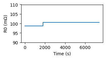
Note how the resistance is corrected very quickly and becomes exact around 1800 seconds, which corresponds to the current pulse. The agreement both shows how online estimators can quickly find the value of parameter values and, importantly, that their accuracy is contingent on whether the data provided allows changes in the model parameters to have a large effect.